Robot Perception with Python: Introduction and Motivation

January 01, 2024 · perception

This is the first post in a series on robotics perception using Python’s standard scientific computing libraries (numpy, scipy, matplotlib). In this series, we will not be using GTSAM or ROS. We will be focusing just on the math from scratch.

The full tutorial repo is available here: Intro to Robot Perception (Python). In order to follow some of the examples, I encourage you to clone the repo. I have added instructions to the bottom of the page.

Why Perception?

A robot that cannot perceive its environment cannot act reliably in it. Perception is the bridge between raw sensor data and meaningful state estimates. The robot needs to be able to answer: where am I, what is around me, and how certain am I?

This series covers that full pipeline: sensors, filtering, localization, mapping, and SLAM.

What is Robotics Perception?

Robotics perception is the field that enables robots to understand and interact with their environment through sensor data. Unlike humans who naturally process visual, auditory, and tactile information, robots must explicitly process sensor measurements to build models of the world around them.

The typical perception pipeline consists of:

Sensing — acquiring data from sensors (cameras, LiDAR, IMU, GPS, etc.)
Preprocessing — filtering, calibration, and initial data processing
Feature Extraction — identifying relevant features in the data
Estimation — combining sensor data to estimate robot state
Mapping — building and maintaining models of the environment
Decision Making — using perception results for control and planning

The Core Problem: Uncertainty

The central challenge in robotics perception is not computation — it is uncertainty. Real robots face two unavoidable sources of it:

Process noise — the robot’s motion model is never perfect. Motors slip, wheels skid, and actuator commands are never executed exactly as specified. Even a simple straight-line command results in a curved path (or almost).

Measurement noise — sensors lie, at least a little. A LiDAR return, a GPS fix, or a camera pixel all carry noise. The world your robot observes is always a noisy version of the real world.

First Example: Simple Robot Motion

Let’s start with the simplest possible case, a robot moving with constant velocity, no noise, no uncertainty:

import numpy as np
import matplotlib.pyplot as plt

# Simple 2D robot motion
def simulate_robot_motion():
    # Robot starts at origin
    x = np.array([0.0, 0.0])  # [x, y] position
    dt = 0.1  # time step
    
    # Store trajectory
    trajectory = [x.copy()]
    
    # Simulate motion for 5 seconds
    for t in np.arange(0, 5, dt):
        # Simple motion model: constant velocity
        velocity = np.array([1.0, 0.5])  # [vx, vy]
        x += velocity * dt
        trajectory.append(x.copy())
    
    return np.array(trajectory)

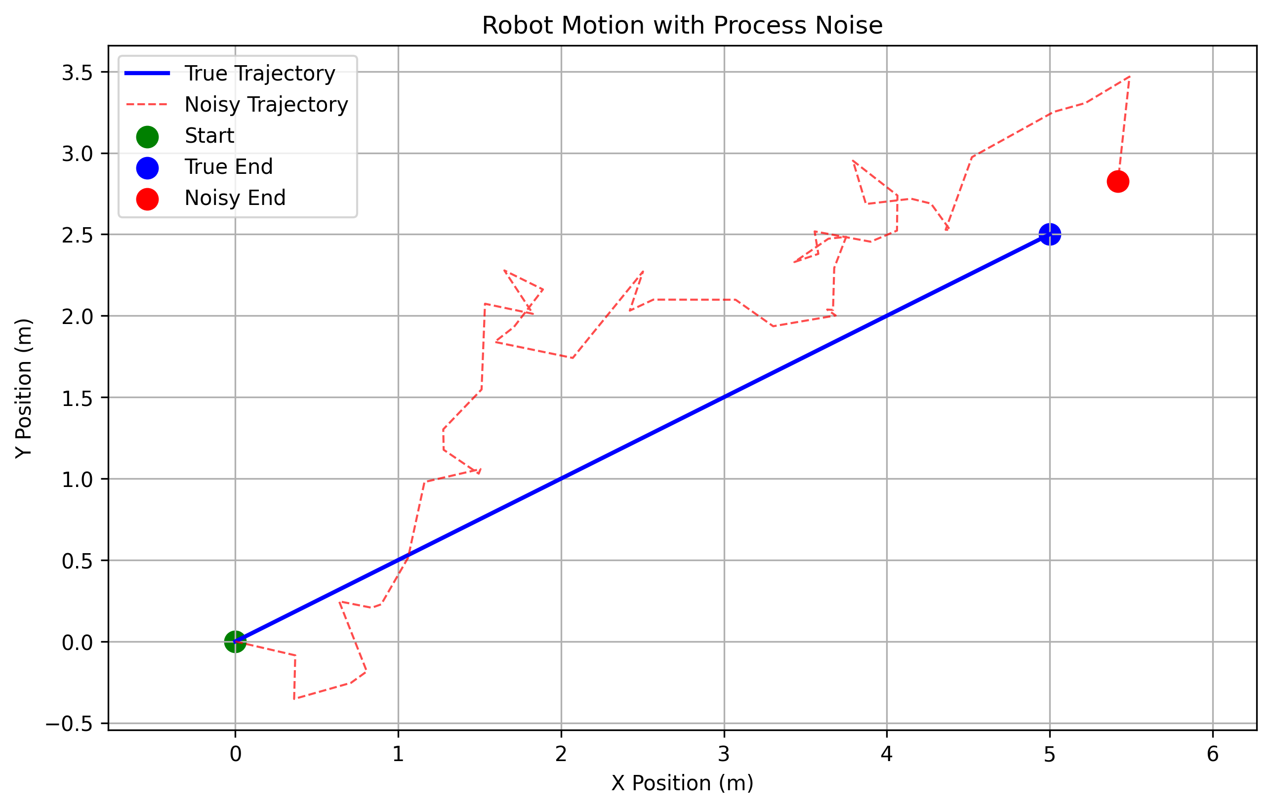
The figure below illustrates what happens when we add noise. The blue line shows this ideal motion, a robot that moves exactly as commanded. The dotted red line shows realistic motion, where each step accumulates a small random error.

Simple vs Noisy Motion

Uncertainty Grows Over Time

The critical insight of this chapter is that uncertainty does not stay constant — it accumulates with time. Each step taken without a corrective sensor measurement adds more uncertainty to the robot’s state estimate.

If the robot’s position at time $t$ is $x_t$ and it takes a step $u_t$ with noise $w_t \sim \mathcal{N}(0, Q)$:

$$ x_{t+1} = x_t + u_t + w_t $$

Then the variance of $x_t$ grows with each step:

$$ \sigma^2_t = \sigma^2_{t-1} + Q $$

This is why filtering algorithms like the Kalman filter exist — they fuse noisy motion predictions with noisy sensor corrections and keep uncertainty bounded within an acceptable range.

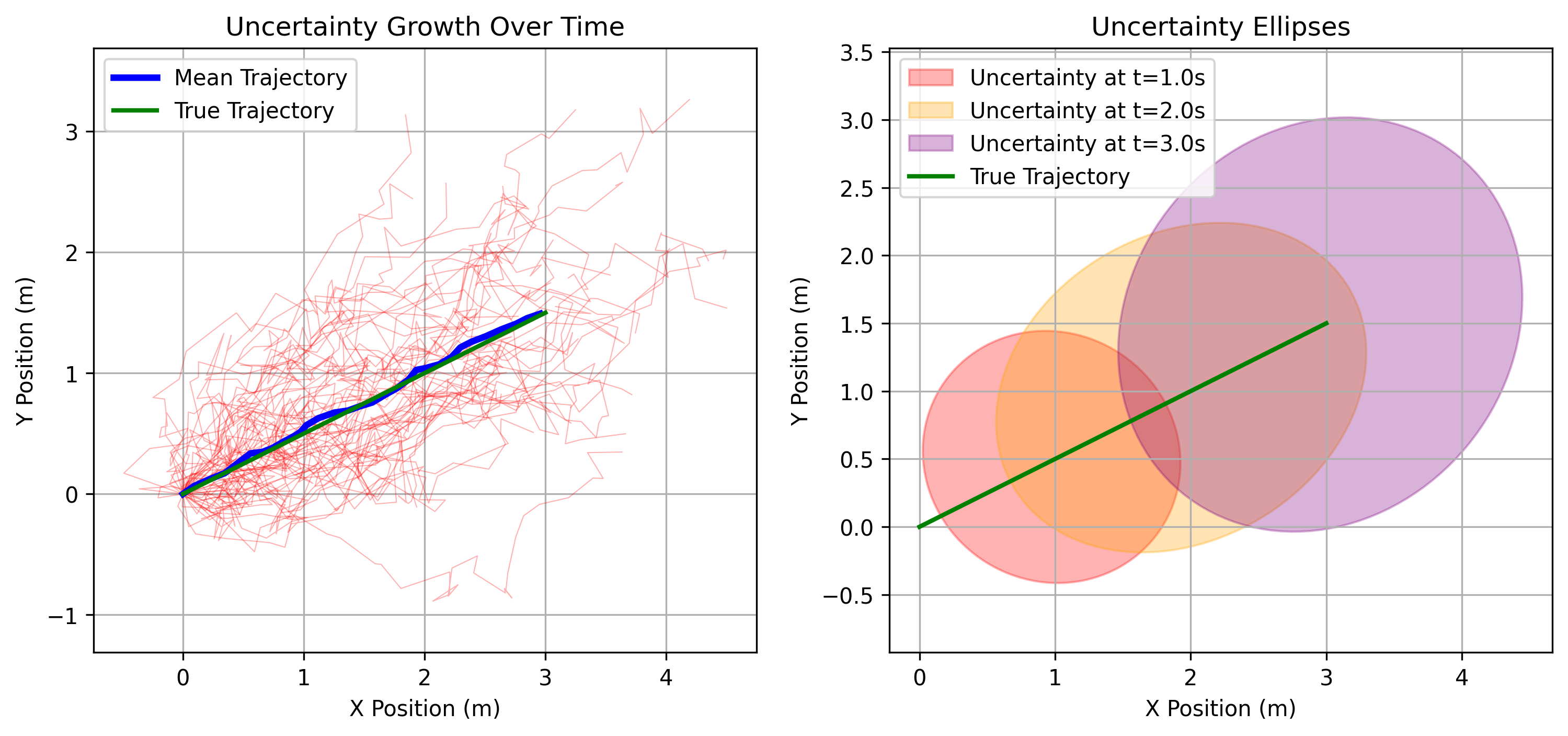
The figure below shows this effect directly. The left plot shows multiple possible robot trajectories in red due to process noise. The right plot shows uncertainty ellipses that represent our confidence in the robot’s position at different times. Notice how they grow larger the further we go without a sensor correction.

Uncertainty Growth

Core Perception Problems

These uncertainty challenges give rise to the central problems this series addresses:

Localization — where am I?
Mapping — what does the environment look like?
SLAM — where am I and what does the environment look like, simultaneously?
Object Detection — what objects are present?
Tracking — how are objects moving?

Why Pure Python?

While libraries like GTSAM, OpenCV, and PCL are powerful tools, they can obscure the underlying mathematics. We are focusing on implementing algorithms from scratch using only NumPy and SciPy so that we can:

Understand the math — every operation is explicit and traceable
Build intuition — see exactly how algorithms work internally
Debug easily — identify exactly where problems occur
Modify freely — adapt algorithms for specific applications

What This Series Covers

Introduction and Motivation ← you are here
Mathematical Foundations
Sensors and Sensor Models
Filtering and Estimation Theory
Localization
Mapping
SLAM
Advanced Perception Algorithms

Prerequisites

Math: linear algebra (vectors, matrices), probability theory (distributions, Bayes’ rule), basic calculus, statistics (mean, variance). We will cover some of these in the next chapter.

Programming: Python basics, NumPy array operations, basic object-oriented programming.

Running the Examples

Clone the repo and install dependencies:

git clone https://github.com/sof-danny/Intro_to_Robot_Perception_Python
cd Intro_to_Robot_Perception_Python
pip install -r requirements.txt

Run the chapter 1 examples individually:

cd chapters/01_introduction
python examples/simple_motion.py
python examples/noisy_motion.py
python examples/uncertainty_growth.py

Or run everything at once:

python examples/complete_demo.py

Exercises

Modify Simple Motion — edit examples/simple_motion.py to include angular velocity and plot orientation over time.
Experiment with Noise — modify examples/noisy_motion.py to test different noise levels. How does increasing the noise standard deviation affect final position error?
Sensor Fusion — create an example that combines GPS and odometry with different noise characteristics. Which sensor should you trust more?
Uncertainty Analysis — extend examples/uncertainty_growth.py to compare uncertainty growth under constant velocity vs. constant acceleration.

Next up: Chapter 2 — Mathematical Foundations, covering the linear algebra, probability theory, and coordinate transforms that every algorithm in this series relies on.