Robot Perception with Python: Mathematical Foundations
January 15, 2024 · perception
This is Chapter 2 of the Robot Perception with Python series. If you haven’t read Chapter 1, start here.
The full code for this chapter is available in the repo:
cd chapters/02_mathematical_foundations
python examples/complete_demo.py
Introduction
Robotics perception relies heavily on mathematical tools for representing uncertainty, transforming between coordinate frames, and processing sensor data. This chapter establishes the foundations that underpin all perception algorithms we’ll develop in subsequent chapters. The examples are organized into focused, modular files:
examples/linear_algebra.py— vector operations, matrices, eigenvalue decompositionexamples/probability.py— probability distributions, Bayes’ rule, statistical momentsexamples/coordinate_transforms.py— 2D/3D transformations, homogeneous coordinatesexamples/estimation.py— least squares, MLE, uncertainty propagation, optimizationexamples/complete_demo.py— comprehensive demonstration
Linear Algebra Essentials
Linear algebra provides the framework for representing and manipulating geometric transformations, sensor data, and uncertainty. In robotics perception, vectors represent positions, velocities, forces, and sensor readings.
Key Vector Operations
| Operation | Description |
|---|---|
| Magnitude | Length of a vector using the Euclidean norm |
| Unit Vector | Magnitude-1 vector pointing in the same direction |
| Dot Product | Measures similarity between two vectors |
| Cross Product | Vector perpendicular to both inputs (3D only) |
import numpy as np

def vector_examples():
    position = np.array([3.0, 4.0, 0.0])
    velocity = np.array([1.0, 2.0, 0.0])

    magnitude    = np.linalg.norm(position)
    unit_vector  = position / magnitude
    dot_product  = np.dot(position, velocity)
    cross_product = np.cross(position, velocity)

    return magnitude, unit_vector, dot_product, cross_product
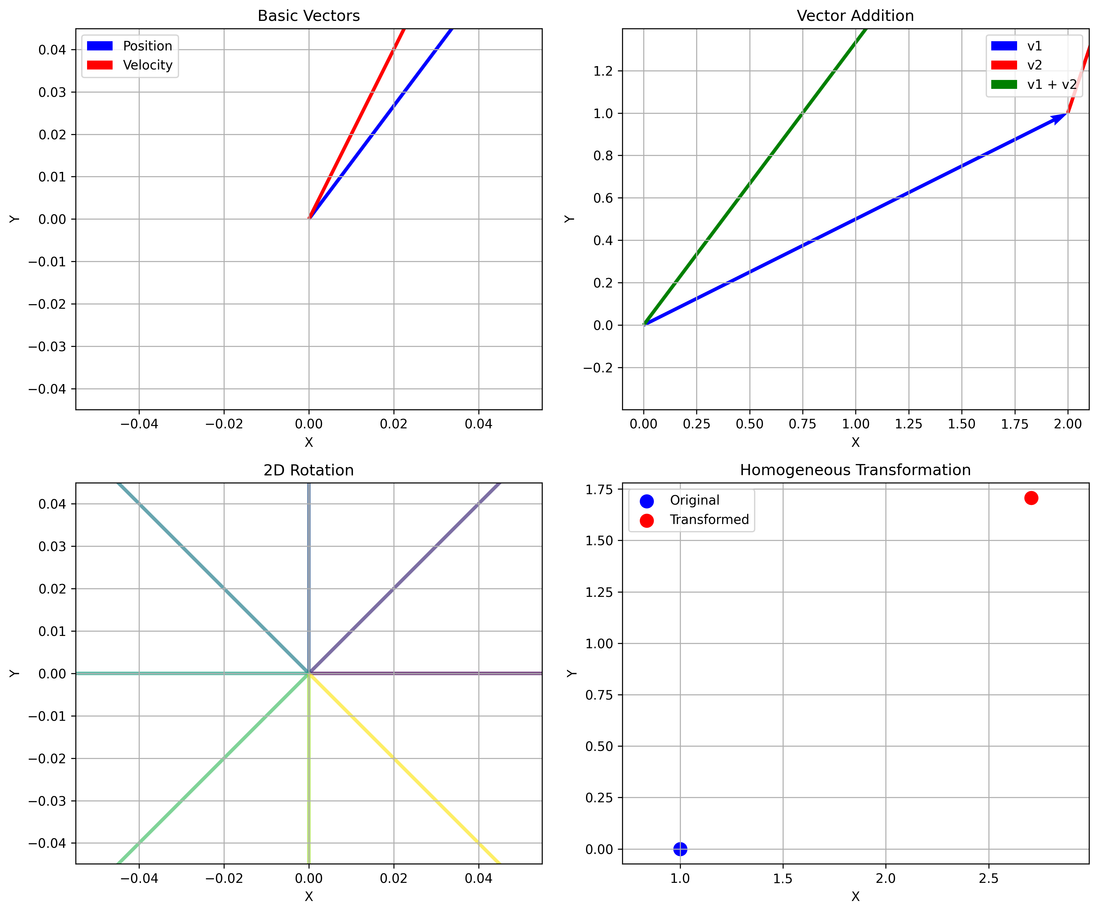
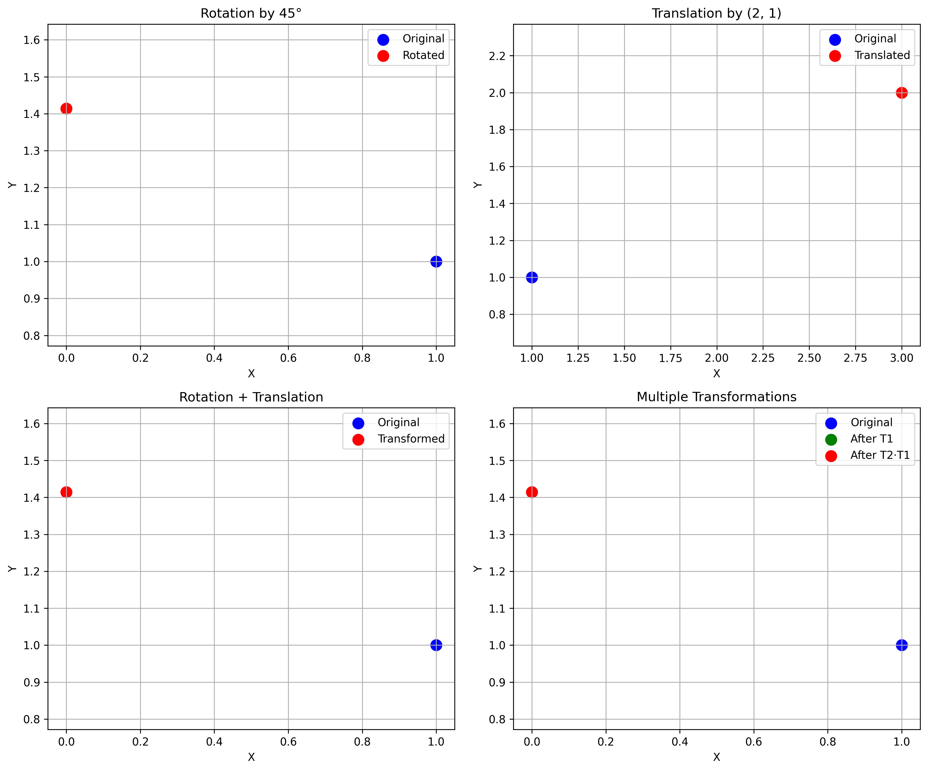
Rotation Matrices
Rotation matrices are orthogonal matrices that represent orientation between coordinate frames. They preserve vector lengths and angles.
Key properties: $R^T R = I$, $\det(R) = \pm 1$, and rotations compose as $R_{total} = R_2 R_1$.
For a 2D rotation by angle $\theta$:
$R(\theta) = \begin{bmatrix} \cos\theta & -\sin\theta \\ \sin\theta & \cos\theta \end{bmatrix}$
def rotation_matrix_2d(angle):
    c, s = np.cos(angle), np.sin(angle)
    return np.array([[c, -s],
                     [s,  c]])

def rotation_matrix_3d(roll, pitch, yaw):
    Rx = np.array([[1, 0,              0           ],
                   [0, np.cos(roll),  -np.sin(roll)],
                   [0, np.sin(roll),   np.cos(roll)]])

    Ry = np.array([[ np.cos(pitch), 0, np.sin(pitch)],
                   [ 0,             1, 0            ],
                   [-np.sin(pitch), 0, np.cos(pitch)]])

    Rz = np.array([[np.cos(yaw), -np.sin(yaw), 0],
                   [np.sin(yaw),  np.cos(yaw), 0],
                   [0,            0,           1]])

    return Rz @ Ry @ Rx  # ZYX convention
Homogeneous Transformations
To handle both rotation and translation in a single matrix operation:
def homogeneous_transform_2d(rotation_matrix, translation):
    T = np.eye(3)
    T[:2, :2] = rotation_matrix
    T[:2, 2]  = translation
    return T

def transform_point(point, T):
    homogeneous = np.append(point, 1)
    return (T @ homogeneous)[:2]
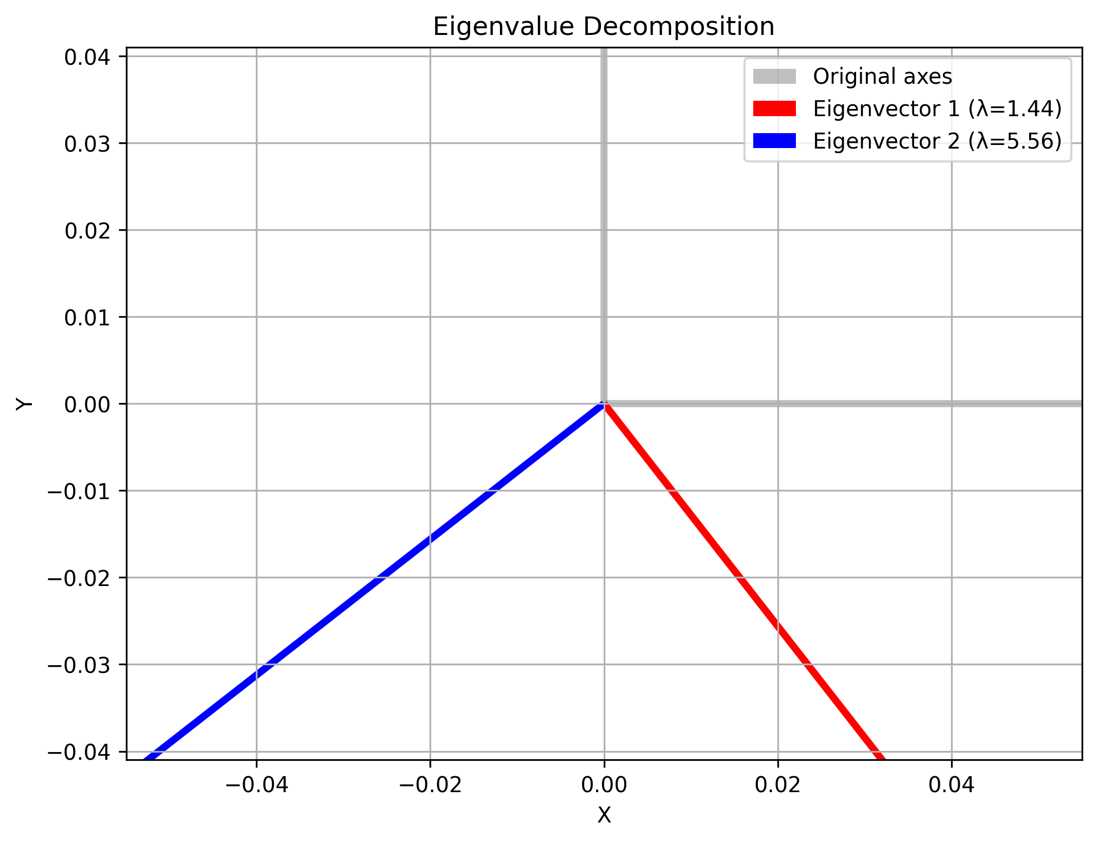
Matrix Decompositions
Eigenvalue Decomposition — useful for analyzing covariance matrices and uncertainty ellipsoids:
def eigenvalue_decomposition_example():
    A = np.array([[4, 2],
                  [2, 3]])
    eigenvalues, eigenvectors = np.linalg.eigh(A)
    reconstructed = eigenvectors @ np.diag(eigenvalues) @ eigenvectors.T
    return eigenvalues, eigenvectors, reconstructed
Singular Value Decomposition (SVD) — useful for least-squares problems and sensor data analysis:
def svd_example():
    A = np.random.rand(5, 3)
    U, S, Vt = np.linalg.svd(A, full_matrices=False)
    reconstructed = U @ np.diag(S) @ Vt
    return U, S, Vt, reconstructed
Probability Theory
Since sensors provide noisy measurements and robot motion is imperfect, we need probabilistic models to represent and reason about uncertainty.
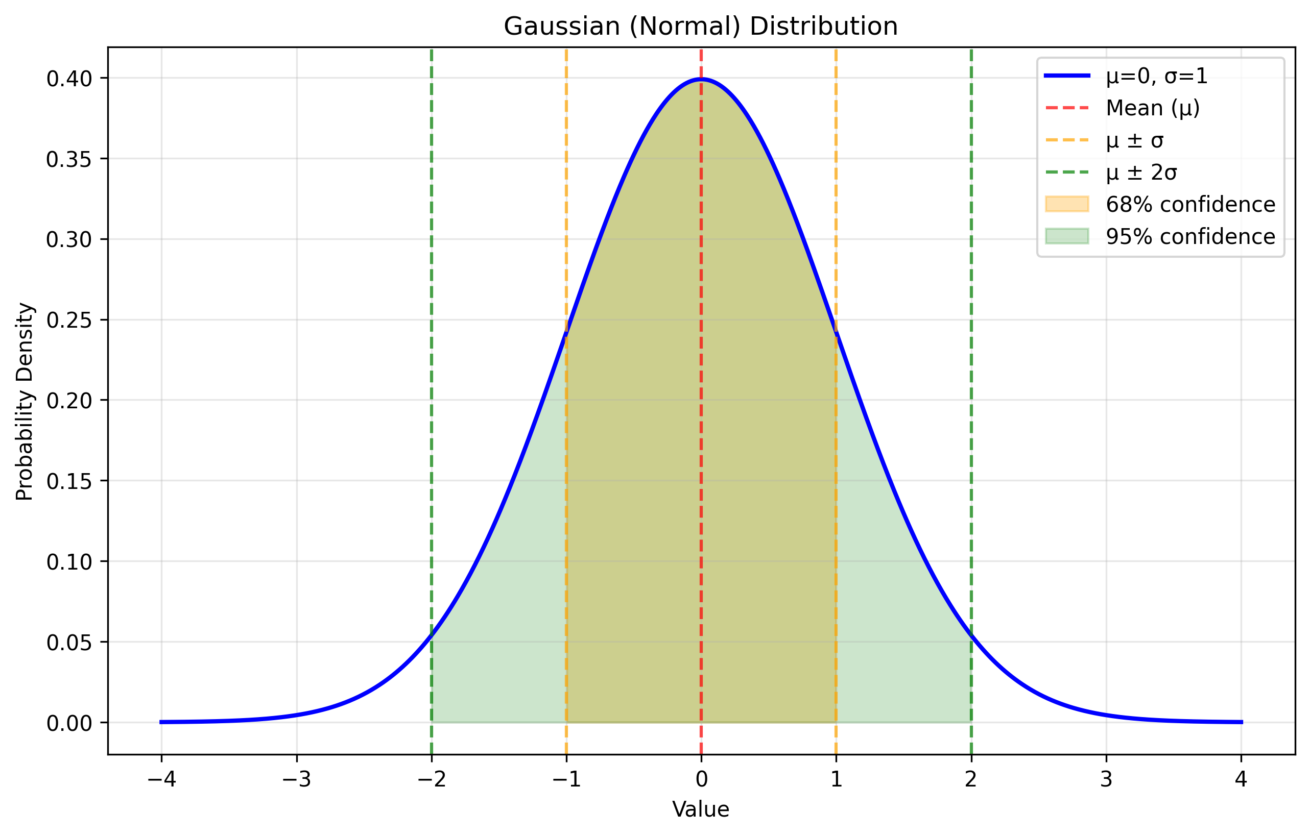
Gaussian Distribution
The Gaussian distribution is the most important distribution in robotics perception. For a univariate Gaussian with mean $\mu$ and variance $\sigma^2$:
Why Gaussians? The Central Limit Theorem guarantees that sums of many random variables tend toward Gaussian distributions. They also remain Gaussian under linear transformations — a crucial property for filtering.
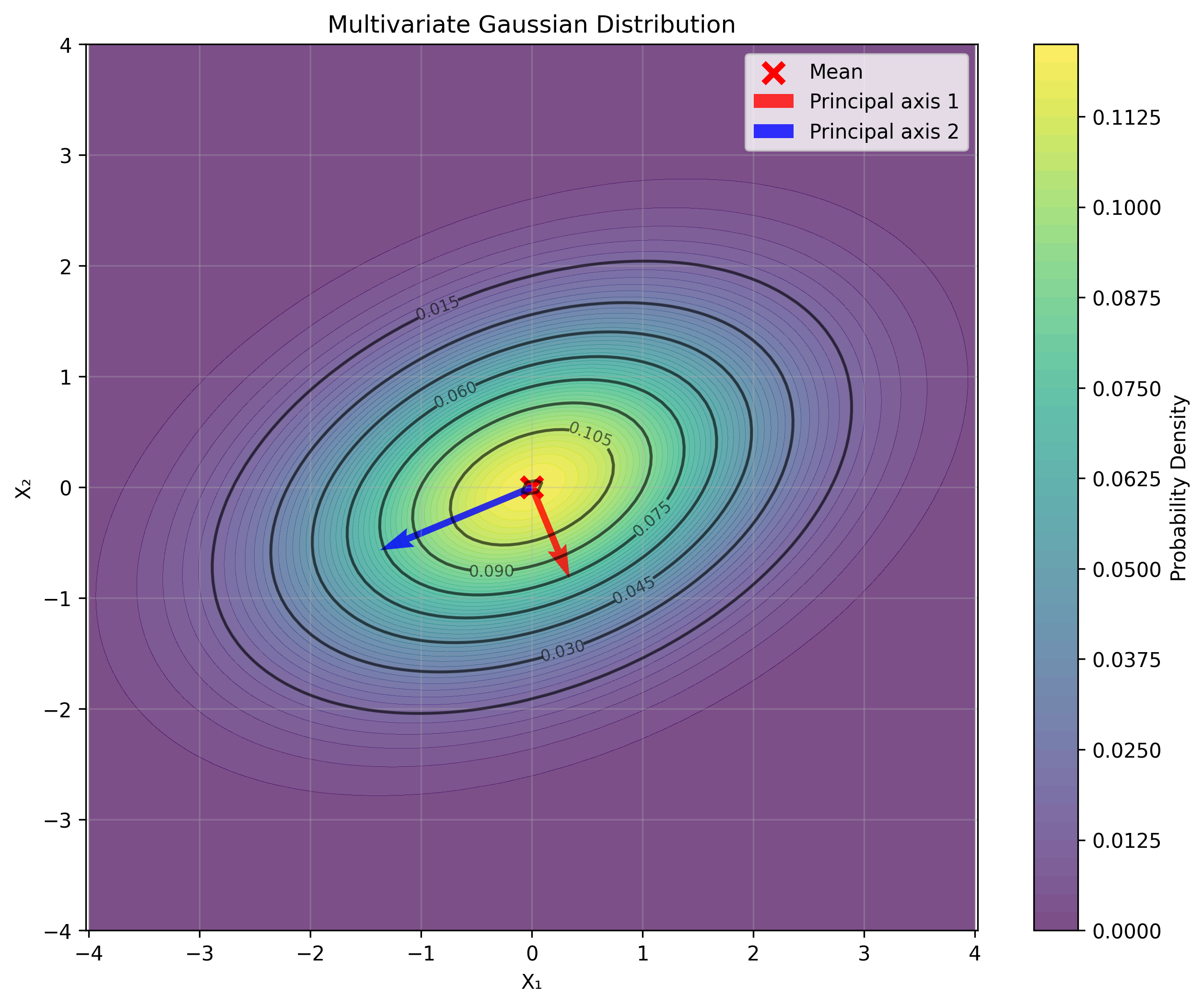
Multivariate Gaussian Distribution
For multiple correlated variables:
where $\boldsymbol{\mu}$ is the mean vector, $\Sigma$ is the covariance matrix, and $k$ is the dimension.
def multivariate_gaussian(x, mean, covariance):
    n = len(x)
    det_cov = np.linalg.det(covariance)
    normalization = 1.0 / np.sqrt((2 * np.pi)**n * det_cov)
    diff = x - mean
    inv_cov = np.linalg.inv(covariance)
    mahalanobis_dist = diff.T @ inv_cov @ diff
    return normalization * np.exp(-0.5 * mahalanobis_dist)

def sample_gaussian(mean, covariance, n_samples=1000):
    L = np.linalg.cholesky(covariance)
    z = np.random.randn(len(mean), n_samples)
    return (mean[:, np.newaxis] + L @ z).T
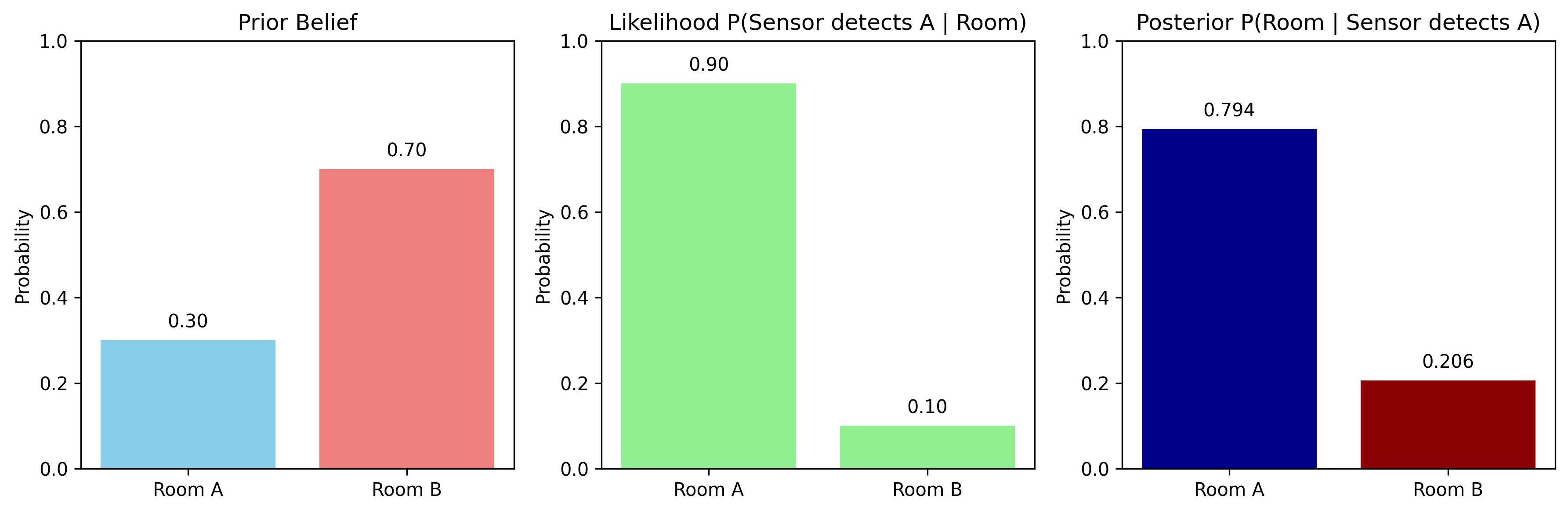
Bayes’ Rule
Bayes’ rule is the foundation of all estimation and filtering in robotics:
where $P(A|B)$ is the posterior (belief after evidence), $P(B|A)$ is the likelihood, $P(A)$ is the prior, and $P(B)$ is the marginal likelihood.
def bayes_rule_example():
    # Prior belief about robot location (4 possible locations)
    prior = np.array([0.1, 0.3, 0.4, 0.2])

    # Likelihood of sensor measurement given each location
    likelihood = np.array([0.8, 0.6, 0.3, 0.1])

    evidence  = np.sum(prior * likelihood)
    posterior = (prior * likelihood) / evidence

    return prior, likelihood, posterior
Uncertainty Propagation
For a linear transformation $\mathbf{y} = A\mathbf{x} + \mathbf{b}$, if $\mathbf{x} \sim \mathcal{N}(\boldsymbol{\mu}_x, \Sigma_x)$, then:
$\boldsymbol{\mu}_y = A\boldsymbol{\mu}_x + \mathbf{b}, \qquad \Sigma_y = A \Sigma_x A^T$
def uncertainty_propagation():
    x_mean = np.array([1.0, 2.0])
    x_cov  = np.array([[0.1, 0.05],
                       [0.05, 0.2]])

    A = np.array([[2, 1],
                  [0, 1]])
    b = np.array([1.0, 0.0])

    y_mean = A @ x_mean + b
    y_cov  = A @ x_cov @ A.T

    return y_mean, y_cov
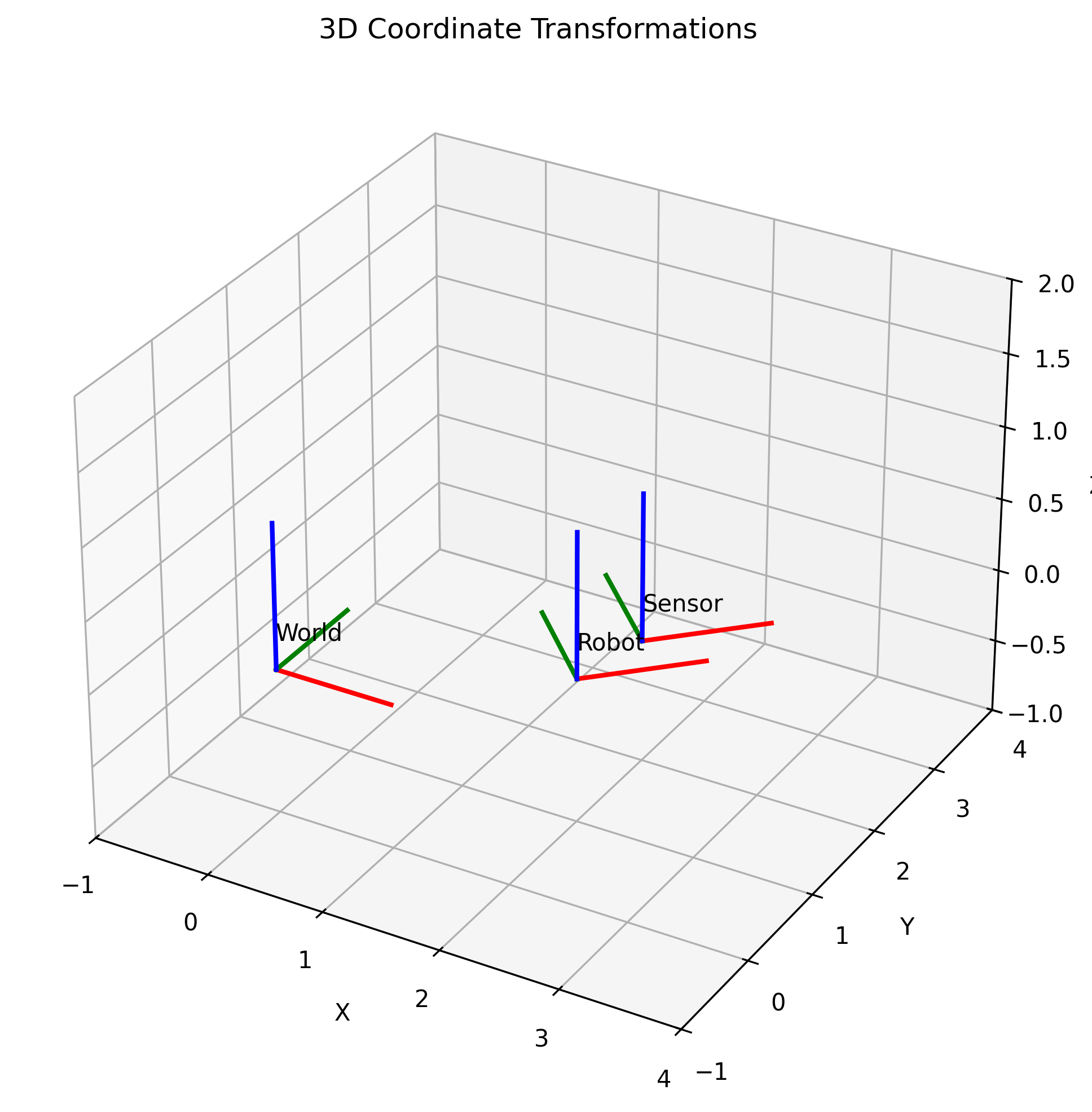
Coordinate Systems and Transformations
Robots operate in physical space and must relate sensor measurements to the world. Coordinate transforms are essential for sensor fusion, localization, mapping, and navigation.
Homogeneous Coordinates
Homogeneous coordinates add an extra dimension to combine rotation and translation into a single matrix:
2D Coordinate Frames
class CoordinateFrame2D:
    def __init__(self, origin, rotation_angle):
        self.origin = np.array(origin)
        self.R = rotation_matrix_2d(rotation_angle)
        self.T = homogeneous_transform_2d(self.R, self.origin)

    def to_world(self, point_local):
        return transform_point(point_local, self.T)

    def to_local(self, point_world):
        return transform_point(point_world, np.linalg.inv(self.T))
3D Coordinate Frames
class CoordinateFrame3D:
    def __init__(self, origin, rotation_matrix):
        self.T = np.eye(4)
        self.T[:3, :3] = rotation_matrix
        self.T[:3, 3]  = origin

    def to_world(self, point_local):
        return (self.T @ np.append(point_local, 1))[:3]

    def to_local(self, point_world):
        return (np.linalg.inv(self.T) @ np.append(point_world, 1))[:3]
Statistical Estimation
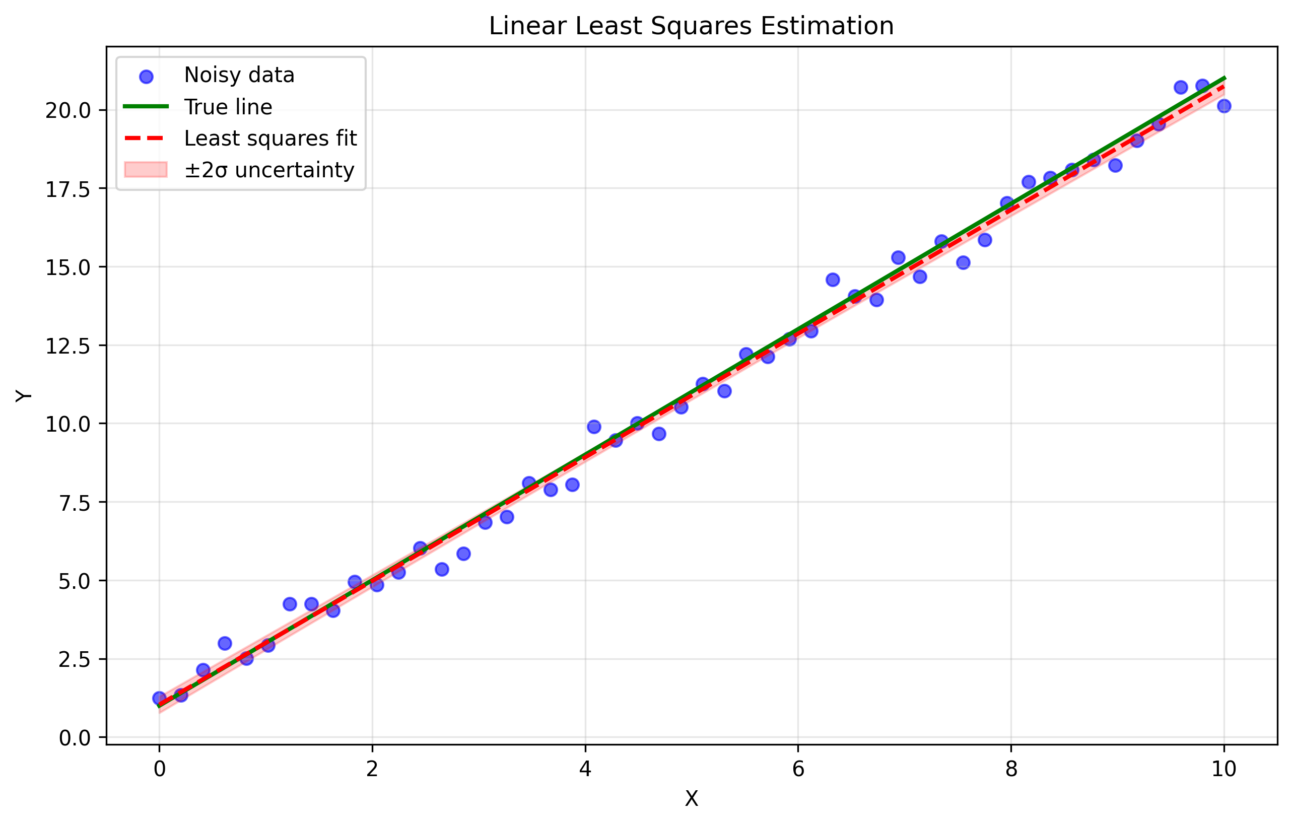
Least Squares
For a linear model $\mathbf{y} = A\boldsymbol{\theta}$, the least squares solution minimizes $|A\boldsymbol{\theta} - \mathbf{y}|^2$:
$\boldsymbol{\theta} = (A^T A)^{-1} A^T \mathbf{y}$
def least_squares_estimation():
    true_m, true_b = 2.0, 1.0
    x = np.linspace(0, 10, 50)
    y = true_m * x + true_b + np.random.normal(0, 0.5, 50)

    A = np.column_stack([x, np.ones(50)])
    params = np.linalg.solve(A.T @ A, A.T @ y)
    m_est, b_est = params

    return true_m, true_b, m_est, b_est
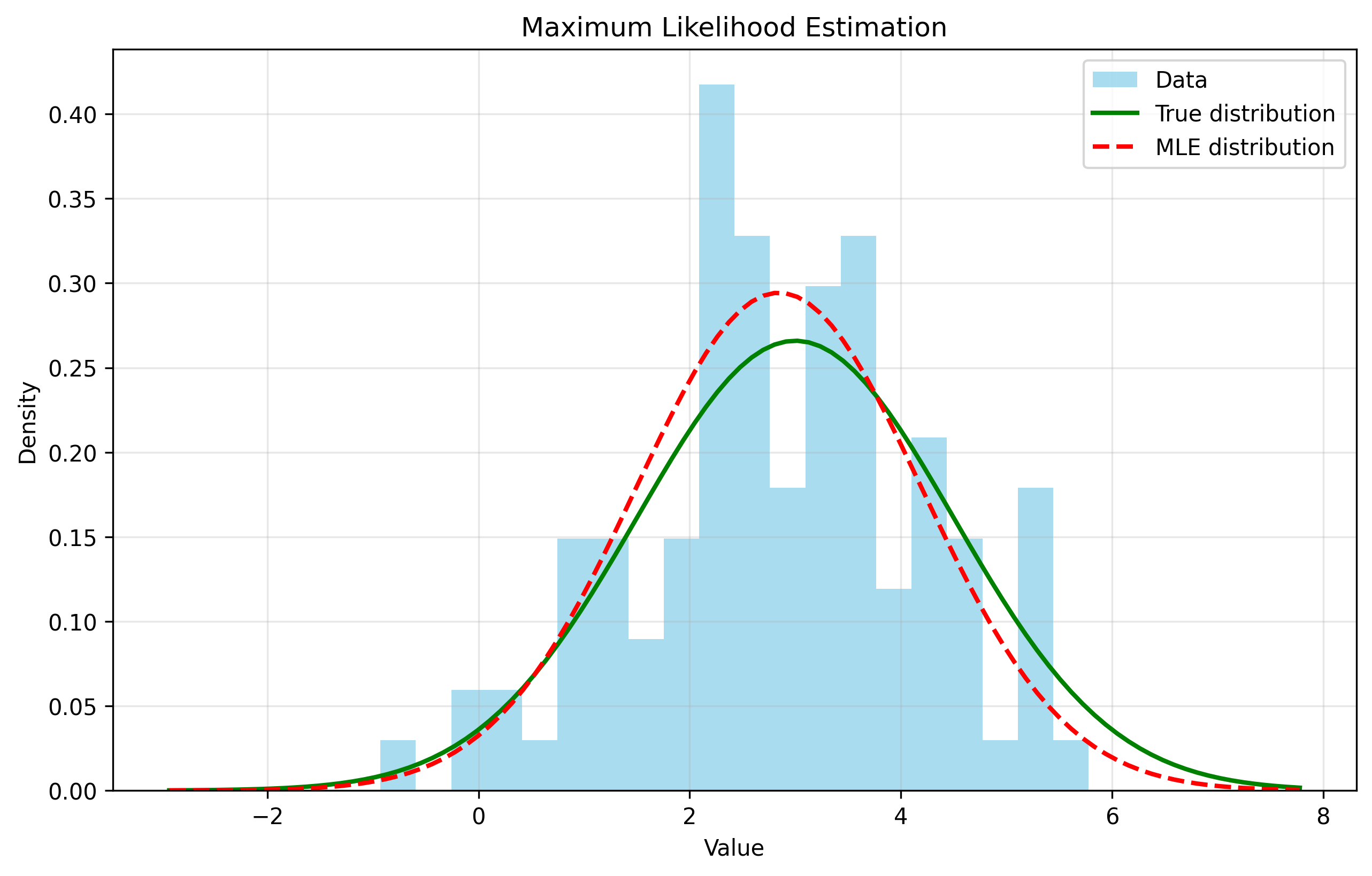
Maximum Likelihood Estimation
MLE finds parameters that maximize $P(\text{data} \mid \boldsymbol{\theta})$:
def maximum_likelihood_estimation():
    true_mean, true_std = 2.0, 1.5
    data = np.random.normal(true_mean, true_std, 100)

    mle_mean = np.mean(data)
    mle_std  = np.std(data, ddof=1)

    return true_mean, true_std, mle_mean, mle_std
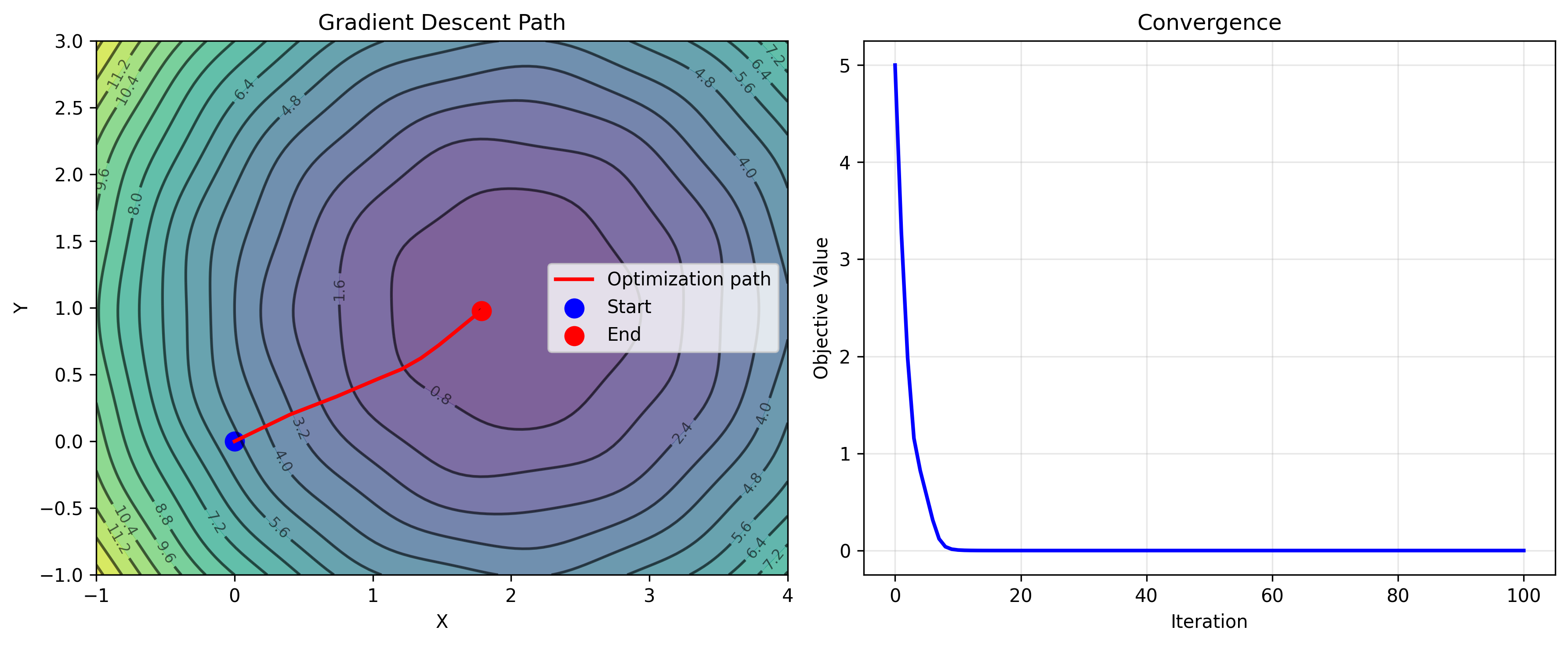
Gradient Descent
For non-linear problems, gradient descent iteratively minimizes an objective:
$\boldsymbol{\theta}_{k+1} = \boldsymbol{\theta}_k - \alpha \nabla f(\boldsymbol{\theta}_k)$
def gradient_descent_example():
    def objective(x): return (x - 2)**2 + 1
    def gradient(x):  return 2 * (x - 2)

    x = 0.0
    lr = 0.1
    history = [x]

    for _ in range(50):
        x = x - lr * gradient(x)
        history.append(x)

    return history, x
Summary
| Topic | Key Tools |
|---|---|
| Linear Algebra | Vectors, rotation matrices, SVD, eigendecomposition |
| Probability | Gaussians, Bayes' rule, covariance matrices |
| Coordinate Systems | Homogeneous transforms, 2D/3D frames |
| Estimation | Least squares, MLE, gradient descent |
Exercises
Basic: Extend linear_algebra.py with vector projection and Gram-Schmidt orthogonalization. Implement functions to check matrix orthogonality and compute QR decomposition.
Intermediate: Implement quaternion representations and conversion from Euler angles. Build an uncertainty propagation example using the unscented transform and compare it to Monte Carlo propagation.
Advanced: Implement Newton’s method and conjugate gradient for optimization. Study the effect of outliers by comparing least squares against RANSAC for line fitting.
Challenge: Build a complete 2D robot tracking pipeline using noisy sensor measurements, a Kalman filter, multiple coordinate frames, and correct uncertainty propagation.
Next up: Chapter 3 — Sensors and Sensor Models, where we’ll look at how to mathematically model the behavior of cameras, LiDAR, and IMUs.